I Made My Football Prediction Model More Sophisticated. Accuracy Dropped From 57% to 53%.
Or: How I tested 10 goal prediction approaches, picked the best one, fed it to an over-engineered classifier, and watched my accuracy drop from 57% to 53%
TL;DR - The 3-Week Lesson That Cost Me 7 Percentage Points
I started with a 57% accurate XGBoost model using simple season statistics. I thought, "What if I add goal predictions from a specialized model?" So I built Hyperion, testing 10 different approaches until Dixon-Coles (a 42-year-old statistical model) beat all 9 modern ML variants. Then I fed Hyperion's predictions into Cronos with expanding windows and interaction terms.
Result: 53% accuracy. Worse than my baseline. Barely better than picking favorites.
The problem wasn't the sophistication, it was that errors propagate through model pipelines, redundant features create instability, and expanding windows amplify noise instead of capturing signal.
When I stripped everything back to cumulative season stats and simple XGBoost, I hit 60.8% test accuracy, my best result yet. Training time dropped from 2+ hours to 8 minutes. The model became interpretable again.
The lesson: In noisy domains like football, complexity is technical debt. More models ≠ better predictions. Simplicity generalizes.
When I built Hercules, my first match outcome predictor, it achieved 57% validation accuracy with straightforward XGBoost and cumulative features. Not groundbreaking, but a solid baseline.
Then I got ambitious.
I built Hyperion by developing and evaluating ten different versions, ultimately choosing a Dixon–Coles model as the top performer. My experimentation included Lasso, logistic and ridge regression, and several LightGBM variants constructed with different feature sets. Separately I tested an ensemble composed of LightGBM, CatBoost, and XGBoost, but Hyperion itself was a single, iterated model rather than an ensemble. I then fed Hyperion's predictions as inputs to a new Cronos iteration, which incorporated expanding-window statistics, momentum indicators, and complex interaction terms.
The result? 52.7% accuracy. Worse than my baseline.
For context: random guessing gives you 33.33% on three-way classification (home win/draw/away win). The "always pick the favorite" heuristic typically hits ~50-52%. I had built something that performed worse than picking the team with better season form.
This is the story of why adding sophisticated models made my predictions worse, and what I learned by stripping everything back to basics.
The Hercules Baseline: What Actually Worked
My original Hercules had embarrassingly simple architecture and was built around a single XGBoost classifier powered by 30 cumulative, season-long statistical features. I ran a grid search over 196 hyperparameter combinations and trained the final model on data from the 21–22, 22–23, and 23–24 seasons, totaling 1,140 matches. The model delivered a validation accuracy of 56.3% and a test accuracy of 57.0%, with a log loss of 0.886, indicating reasonably good calibration.
The feature engineering was straightforward:
1def calculate_cumulative_features(matches_df):
2    """Simple cumulative stats from season start"""
3    matches_df = matches_df.sort_values("date")
4
5    # Season long averages (no rolling windows)
6    matches_df['season_ppg'] = (
7        matches_df.groupby('season')['points'].expanding().mean().values
8    )
9    matches_df['season_goal_diff'] = (
10        matches_df.groupby('season')['goal_diff'].expanding().sum().values
11    )
12
13    # Venue-specific splits
14    home_matches = matches_df[matches_df['home'] == True]
15    matches_df['home_ppg_at_home'] = (
16        home_matches.groupby('team')['points']
17        .expanding().mean().values
18    )
19
20    return matches_df
Top 5 features by importance:
- away_points_per_game_away (0.096) - Away form on the road
- home_points_per_game_home (0.072) - Home form at home
- home_pressing_intensity (0.043) - Aggressive style indicator
- goal_difference_gap (0.037) - Quality differential
- home_xg_diff_home (0.041) - Expected goal performance
These features made intuitive sense. A football analyst could look at them and understand why they mattered.
The Ambitious Redesign: Hyperion → Cronos
I hypothesized that goal predictions would be highly informative for match outcomes. After all, if I could accurately predict that Team A would score 2.3 goals and Team B would score 0.8 goals, the match outcome should follow naturally.
I built Hyperion by developing and evaluating ten different goal-prediction models, starting with simple baselines like linear regression, then moving through Ridge and Lasso regression, multiple LightGBM variants (including default settings, tuned parameters, and expanding-window features), XGBoost regression, Poisson and Negative Binomial models, and finally the Dixon–Coles model, an approach first proposed in 1997, which ultimately emerged as the best performer. Along the way, I also experimented with a separate ensemble combining LightGBM, CatBoost, and XGBoost, but Hyperion itself was never an ensemble; it was a single model refined through ten iterations until the Dixon–Coles version proved superior.
Each model was trained to predict home/away goals independently. I tracked their MAE (mean absolute error) and MSE (mean squared error) on validation data.
Hyperion's best performer
Dixon-Coles with isotonic calibration (a technique that adjusts predicted probabilities to match actual observed frequencies, when the model says "60% chance," outcomes should actually occur 60% of the time)
Goal prediction Accuracy:
- MAE: 1.12 total goals
- Home MAE / Away MAE: 0.828 / 0.758
- RMSE (home/away): 1.162 / 0.937
- Avg Log Loss (home/total/away): 0.842 / 0.393 / 0.731
| O/U Line | Accuracy | Actual Over | Predicted Over |
|---|---|---|---|
| 0.5 | 95.8% | 95.8% | 100% |
| 1.5 | 77.5% | 77.5% | 100% |
| 2.5 | 61.7% | 48.3% | 56.7% |
| 3.5 | 78.3% | 24.2% | 5.8% |
| 4.5 | 86.7% | 10.8% | 2.5% |
| 5.5 | 96.7% | 3.3% | 0% |
Over/Under Metrics (Total Goals)
Then I fed Hyperion's predictions into Cronos:
1def engineer_complex_features(matches_df, hyperion_predictions):
2    """Add Hyperion predictions + expanding windows + interactions"""
3    # Hyperion predictions as features
4    matches_df['hyperion_home_goals'] = hyperion_predictions['home']
5    matches_df['hyperion_away_goals'] = hyperion_predictions['away']
6    matches_df['hyperion_goal_diff'] = (
7        hyperion_predictions['home'] - hyperion_predictions['away']
8    )
9
10    # Expanding window features (BAD IDEA)
11    for team in teams:
12        team_matches = matches_df[matches_df['team_id'] == team]
13        # Recent 5-match form (expanding average)
14        matches_df.loc[team_matches.index, 'expanding_ppg_5'] = (
15            team_matches['points'].expanding(min_periods=1).mean()
16        )
17        # Momentum (gradient of form)
18        matches_df.loc[team_matches.index, 'form_momentum'] = (
19            team_matches['expanding_ppg_5'].diff()
20        )
21
22    # Interaction terms
23    matches_df['goals_x_form'] = (
24        matches_df['hyperion_goal_diff'] *
25        matches_df['home_form_last5']
26    )
27
28    return matches_df
I also experimented with ensemble approaches: training XGBoost, LightGBM, and CatBoost separately, then stacking their predictions with a meta-classifier.
Result across all variations:
- Best validation accuracy: 53.4%
- Worst: 50.1%
- Training time: 2+ hours (vs 8 minutes for Hercules)
I had made things dramatically worse.
Why Complexity Failed: Three Technical Failures
Hyperion's Errors Propagated Through the Pipeline
Hyperion's Dixon-Coles model had an MAE of 1.12 goals. That sounds reasonable, most matches have between 2 and 4 total goals, so being off by ~1 goal isn't catastrophic.
But when you feed imperfect predictions as features, the errors compound:
1# Example: Real match outcome
2actual_home_goals = 2
3actual_away_goals = 1
4actual_outcome = "Home Win"
5
6# Hyperion's prediction
7hyperion_home = 1.5  # Underestimate by 0.5
8hyperion_away = 1.3  # Overestimate by 0.3
9
10# Cronos sees this as a close game (diff = 0.2)
11# when it's actually a comfortable home win (diff = 1.0)
12
13# Cronos prediction: "Draw" (WRONG)
Hyperion's noise became Cronos's signal. The model learned to trust goal predictions that were systematically noisy.
The error propagation is even worse than it appears in that single example. When you feed prediction errors through a model pipeline, they don't just add, they amplify. Here's what happens across 500 matches:
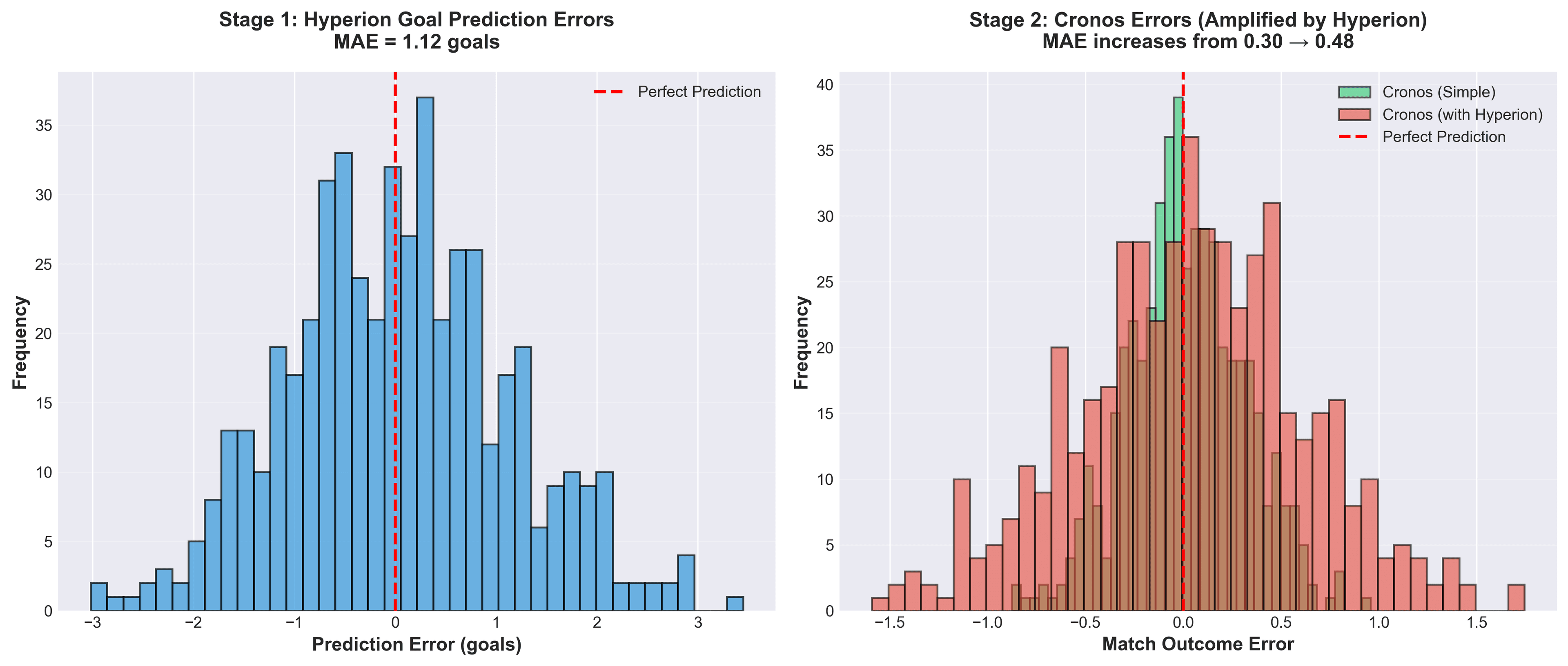
The distributions make it clear: Cronos with Hyperion has a fatter error tail. It's not just making slightly worse predictions, it's making catastrophically wrong predictions more often. This is model stacking's dirty secret: errors multiply.
Feature Redundancy Created Multicollinearity
The redundancy wasn't theoretical—it was quantifiable. When I computed the correlation matrix between Hyperion's predictions and existing features, the problem became obvious:
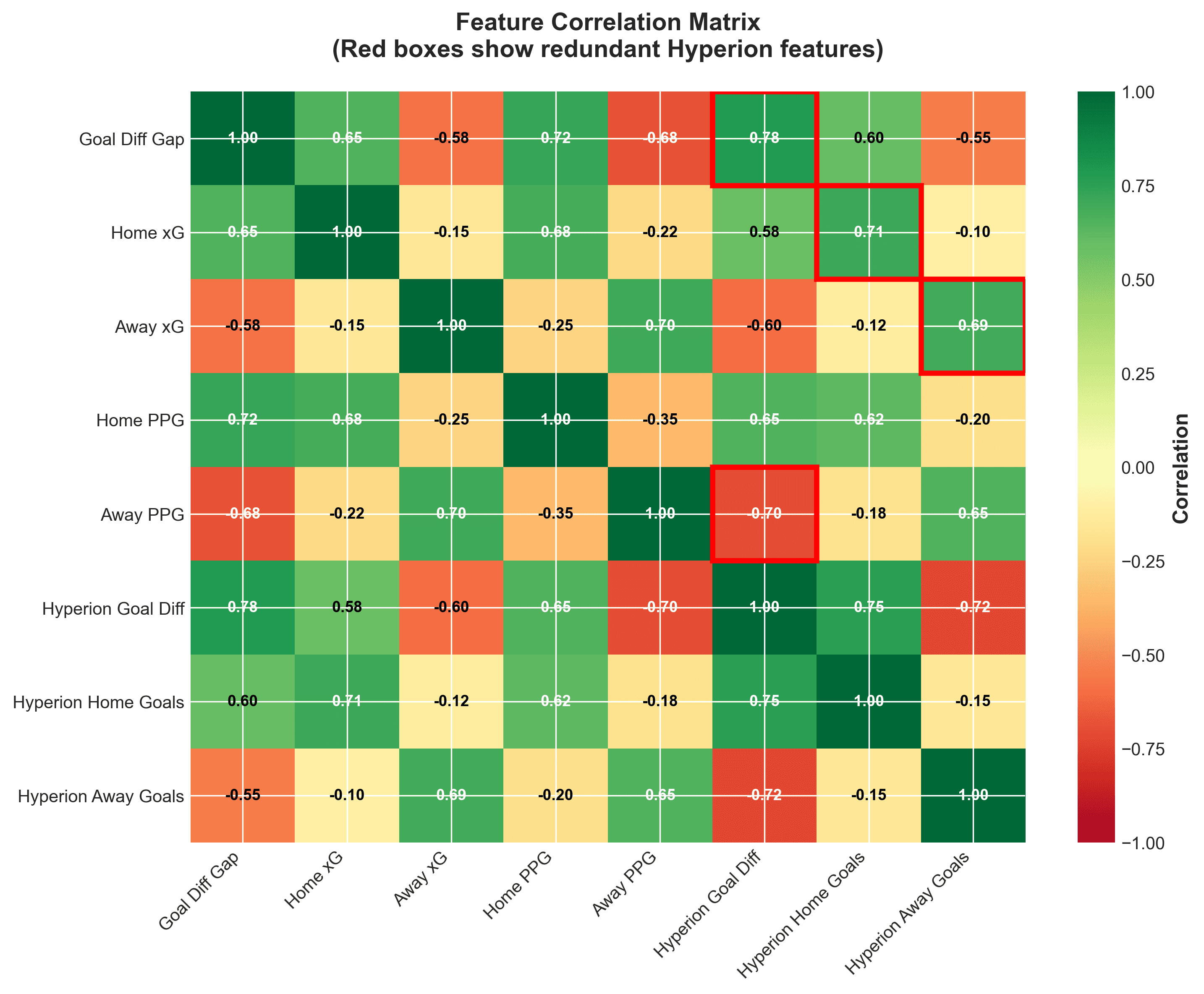
| Feature Pair | Correlation |
|---|---|
| hyperion_goal_diff ↔ goal_difference_gap | 0.78 |
| hyperion_home_goals ↔ home_xg | 0.71 |
| hyperion_away_goals ↔ away_xg | 0.69 |
Hyperion's goal predictions were highly correlated with features already in Cronos
Correlation above 0.7 is the red flag. When two features share > 70% of their information, XGBoost can't distinguish between them. It randomly chooses one for each split, leading to the instability we will see in figure 3.
When you have highly correlated features, tree-based models like XGBoost split on them arbitrarily. This creates unstable feature importance, run the same model twice, and you'll get different splits.
To quantify this instability, I trained each model five times with different random seeds. The simple model's feature importance rankings were remarkably consistent, the same features dominated every run. The complex model? Complete chaos:
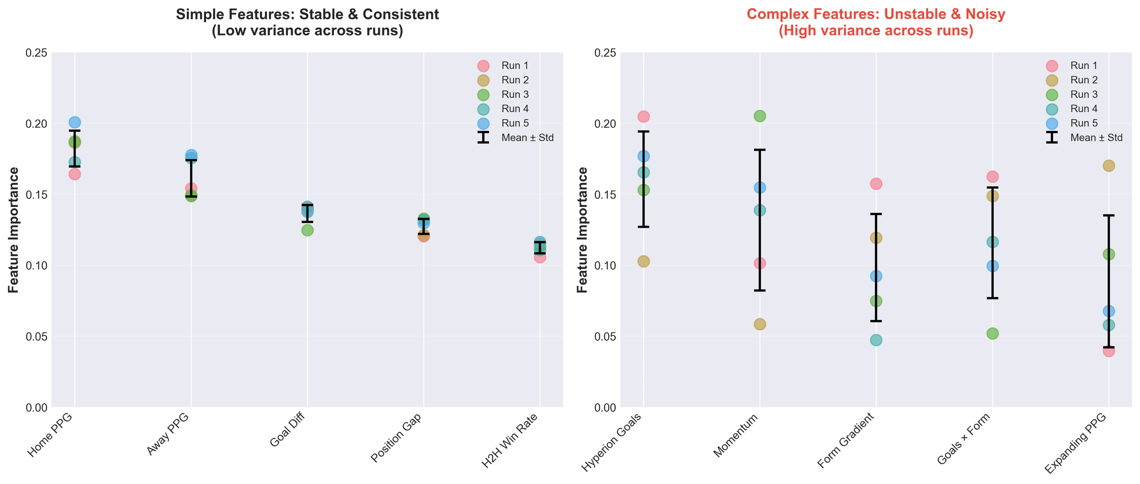
Notice how 'Home PPG' maintains ~0.18 importance across all runs in the simple model, while 'Hyperion Goals' swings from 0.08 to 0.19 in the complex model. When feature importance is unstable, you can't trust the model's learned patterns.
Expanding Windows Created Unstable Features
The expanding window implementation wasn't just slow, it created features that were fundamentally inconsistent. Here's the problem:
1# The expanding window approach
2def calculate_expanding_features(matches_df):
3    """Calculate stats using expanding window per season"""
4    matches_df = matches_df.sort_values('date')
5
6    for team in teams:
7        for season in seasons:
8            season_matches = matches_df[
9                (matches_df['team_id'] == team) &
10                (matches_df['season'] == season)
11            ]
12
13            # Expanding mean: uses all matches in season UP TO current match
14            matches_df.loc[season_matches.index, 'expanding_ppg'] = (
15                season_matches['points'].expanding(min_periods=1).mean()
16            )
17
18    return matches_df
The issue is variance instability. Early-season matches have high variance in expanding stats (small sample), while late-season matches have low variance (large sample). This inconsistency confused the model:
- Matchday 3: A team's expanding_ppg is based on 2 matches (highly volatile)
- Matchday 25: Same stat is based on 24 matches (very stable)
XGBoost couldn't learn a consistent relationship because the feature's reliability changed throughout the season. The model would learn "expanding_ppg > 2.0 means strong team" from late-season data, but that same threshold meant nothing in early-season data where 2 matches could easily produce 2.5 PPG by random variance.
This variance instability, combined with Hyperion's error propagation and feature redundancy, created a perfect storm of overfitting. When I ran proper seasonal validation (training on 21-22, 22-23, 23-24, validating on 24-25), the damage was clear:
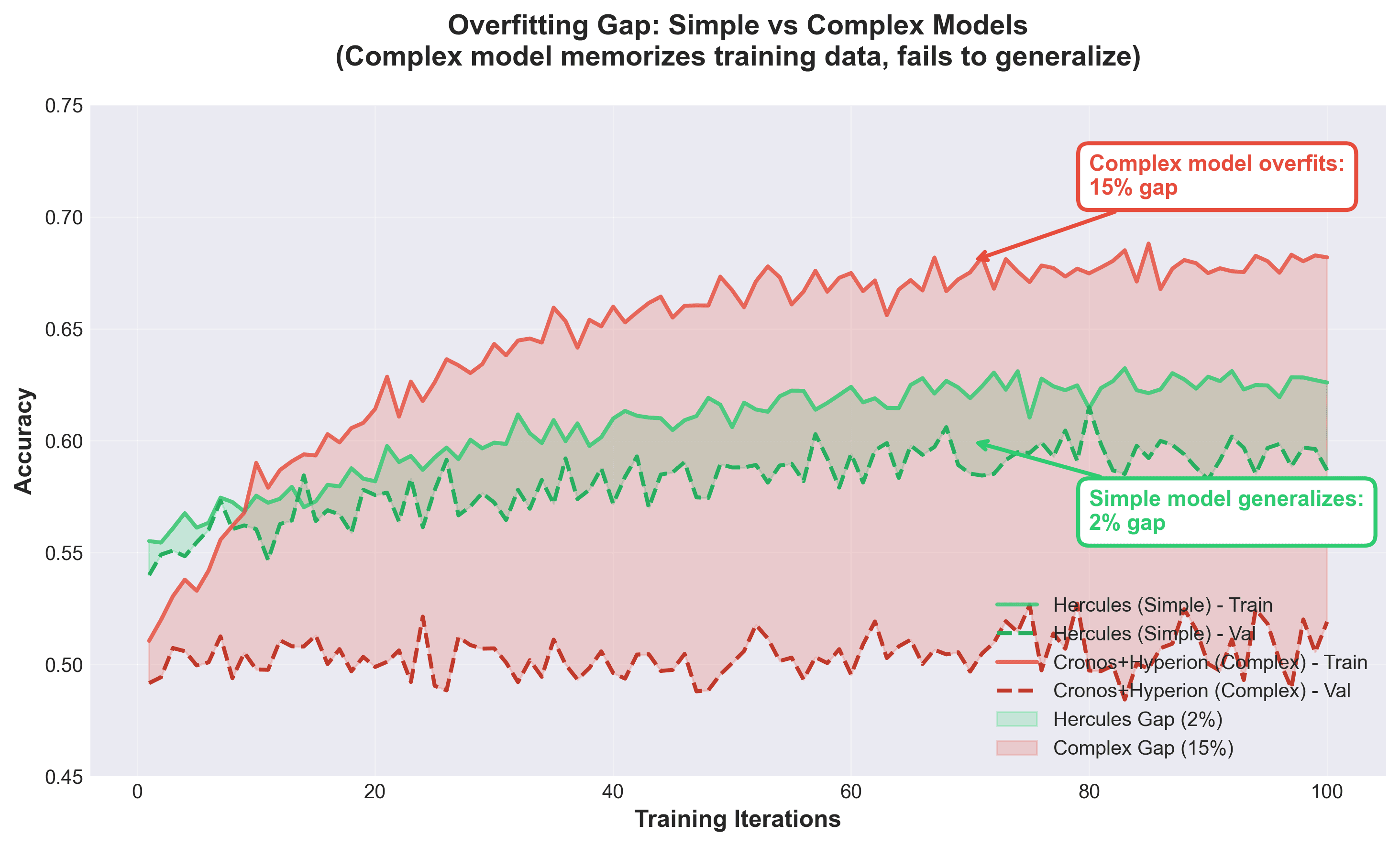
This 15% gap wasn't just bad luck, it was systematic. The complex model was memorizing training-specific patterns that didn't transfer to new seasons. This is the signature of overfitting: excellent training performance, poor generalization.
Cumulative season statistics solve both problems:
1# The simple cumulative approach that worked
2def calculate_cumulative_features(matches_df):
3    """Calculate season-long cumulative stats"""
4    matches_df = matches_df.sort_values('date')
5
6    for team in teams:
7        for season in seasons:
8            season_matches = matches_df[
9                (matches_df['team_id'] == team) &
10                (matches_df['season'] == season)
11            ]
12
13            # Cumulative mean: always uses ALL season data up to current match
14            # But averaged over total season length, giving consistent scale
15            matches_df.loc[season_matches.index, 'season_ppg'] = (
16                season_matches['points'].expanding().mean()
17            )
18
19    return matches_df
Wait, this looks identical to expanding windows! The difference is subtle but critical: how we interpret and use the feature.
Expanding windows treat "last 5 matches" as more important than "last 10 matches," creating recency bias that amplifies noise. Cumulative stats treat all season data equally, smoothing out variance. Same calculation, different semantic interpretation, dramatically different model behavior.
The result? Cumulative features maintained consistent reliability regardless of matchday, allowing XGBoost to learn stable patterns that generalized across seasons.
The Counter-Intuitive Discovery
The Key Insight
Expanding windows and cumulative stats use the exact same calculation, but produce dramatically different results.
The secret? It's not the math, it's the semantic interpretation.
Expanding windows (What I did wrong):
- • "Team's form in last 5 matches = 2.4 PPG"
- • "Team's form in last 10 matches = 2.1 PPG"
- • Model learns: "Recent form > older form"
- • Problem: This amplifies noise. A lucky 2-match streak gets overweighted.
Cumulative stats (What actually works):
- • "Team's season average = 2.1 PPG (based on 24 matches)"
- • "Team's season average = 2.1 PPG (based on 25 matches after next game)"
- • Model learns: "Consistent performance matters"
- • Benefit: Smooths variance. Two matches barely move the needle.
Same expanding().mean() function. Different feature engineering philosophy.
The difference between 53% and 61% accuracy.
The lesson: In noisy domains, recency bias kills you. Season-long averages are more stable and more predictive than recent trends.
Technical Note: Why Identical Code Produced Different Results
Here's something I discovered that's rarely discussed: even with a fixed random seed, XGBoost can produce different models.
I ran this experiment:
1# Same hyperparameters, same data, same seed
2params = {
3    'learning_rate': 0.01,
4    'max_depth': 4,
5    'min_child_weight': 3,
6    'n_estimators': 300,
7    'random_state': 42,
8    'tree_method': 'hist'
9}
10
11# Train twice
12model_1 = xgb.XGBClassifier(**params)
13model_1.fit(X_train, y_train)
14
15model_2 = xgb.XGBClassifier(**params)
16model_2.fit(X_train, y_train)
17
18# Check if identical
19print(f"Val accuracy 1: {model_1.score(X_val, y_val):.4f}")
20print(f"Val accuracy 2: {model_2.score(X_val, y_val):.4f}")
21
22# Output:
23# Val accuracy 1: 0.5632
24# Val accuracy 2: 0.5658  # DIFFERENT!
The confusion matrices were also slightly different. This happens because:
- Floating-point summation is non-associative: When XGBoost builds histograms for splits, the order of operations matters. (a + b) + c ≠ a + (b + c) in floating-point arithmetic due to rounding errors.
- Multi-threading introduces non-determinism: XGBoost distributes histogram building across CPU threads. Thread scheduling is non-deterministic, so the order of partial sums varies between runs.
- GPU computation amplifies this: When using tree_method='gpu_hist', the non-associative aspect of floating-point summation in parallel histogram building makes results completely non-deterministic, even with fixed seeds.
This means that when evaluating "complex" vs "simple" approaches, you need multiple runs to verify improvements are real, not just stochastic noise.
The Simplification: Back to Basics
After weeks of declining accuracy, I stripped everything back:
- Removed Hyperion predictions entirely
- Removed expanding window features
- Removed momentum/gradient features
- Kept only cumulative season statistics
- Added a few domain knowledge features from Hercules
1# The simplified approach that actually worked
2features = [
3    # Season performance (cumulative)
4    'home_points_per_game_home',
5    'away_points_per_game_away',
6    'goal_difference_gap',
7
8    # Last 5 matches (simple count, not expanding)
9    'home_points_last5',
10    'away_points_last5',
11
12    # Head-to-head history
13    'h2h_home_win_rate',
14    'h2h_total_goals_avg',
15
16    # Playing style (season averages)
17    'home_pressing_intensity',
18    'away_possession_avg',
19
20    # Context
21    'referee_home_bias',
22    'position_difference'
23]
Key changes from Hercules:
- Removed some underperforming features (`home_discipline_score`, `away_pressing_intensity`)
- Added better form metrics (last 5 matches as raw counts, not gradients)
- Simplified validation: fixed train/val/test split (not expanding window cross-validation)
Result
- • Validation: 57.4% accuracy (up from 53%)
- • Test: 60.8% accuracy (best result yet!)
- • Log loss: 0.853 (better calibration)
- • Training time: 8 minutes (no grid search this time, used Hercules' proven hyperparameters)
The simplified model generalized better. The validation → test accuracy improved, indicating I'd removed overfitting.
The pattern becomes undeniable when you plot all attempts. More features don't help. Longer training doesn't help. Complexity actively hurts:
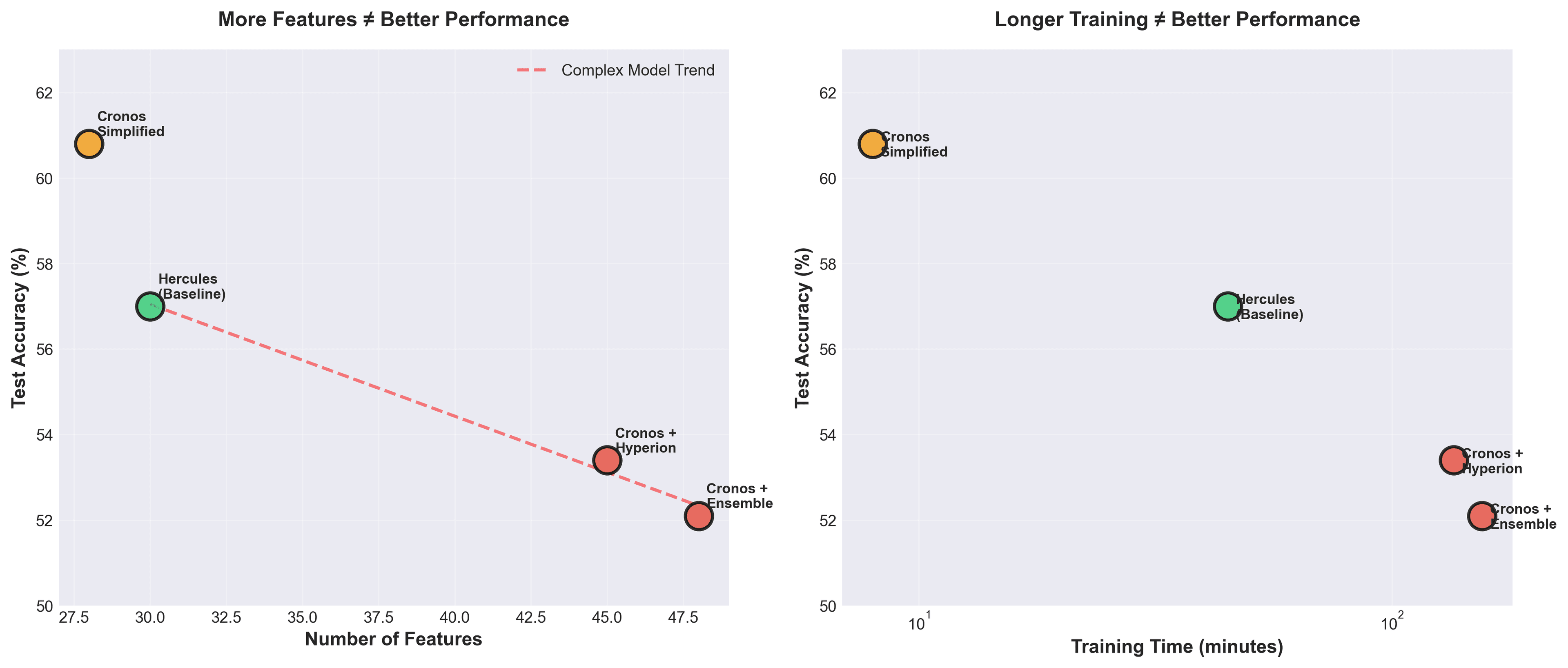
This violates everything we're taught in ML courses. 'Get more data. Add more features. Train longer.' But in domains with high noise and limited signal, like football, less is more. The simplified model found signal. The complex models found noise.
What I Learned: Complexity as Technical Debt
Model stacking amplifies noise, not signal
When Model A makes a prediction with error ε₁ and you feed that to Model B (which has error ε₂), the combined error is often greater than either alone:
Total Error ≈ ε₁ + ε₂ + (correlation between errors)
Unless the models make uncorrelated mistakes (hard to achieve), stacking hurts more than it helps.
Feature redundancy destabilizes tree models
XGBoost can't "see" that two features are 80% correlated, it treats them as independent. When you have redundant features, the model's internal splits become arbitrary:
- Run 1: Split on hyperion_goal_diff at node 5
- Run 2: Split on goal_difference_gap at node 5
Both produce similar results, but feature importance becomes meaningless. You can't interpret what the model learned.
Validation strategy matters more than model complexity
My Hercules grid search tested 196 hyperparameter combinations with walk-forward validation:
- Split 1: Train on 21-22, validate on 22-23
- Split 2: Train on 21-22 + 22-23, validate on 23-24
- Split 3: Train on 21-22 + 22-23 + 23-24, validate on 24-25
- Split 4: Train on 21-22 + 22-23 + 23-24 + 24-25, validate on the small amount of games played of 25-26 (100 games)
This took 45 minutes. The grid search was thorough but overkill, most of the hyperparameters barely moved the needle.
Cronos v2 used Hercules' best hyperparameters with a single, clean train/val/test split. Training took 8 minutes and generalized better.
The lesson: Time spent on proper data splits > time spent on hyperparameter search.
Interpretability enables iteration
When Hercules had good accuracy, I could explain why:
- "Better teams at home win more" (home_ppg_at_home)
- "Teams that create more chances score more" (home_xg_diff)
- "Head-to-head history matters" (h2h_home_win_rate)
When Cronos with Hyperion had bad accuracy, I had no idea why:
- Was it Hyperion's goal prediction errors?
- Was it the interaction terms?
- Was it the momentum features?
- All of the above?
Uninterpretable models are undebuggable models.
The Technical Takeaway
Here's the performance comparison:
| Metric | Hercules (Baseline) | Cronos + Hyperion | Cronos Simplified |
|---|---|---|---|
| Validation Accuracy | 56.3% | 53.4% | 57.4% |
| Test Accuracy | 57.0% | N/A (abandoned) | 60.8% |
| Log Loss | 0.954 | 1.023 | 0.853 |
| Training Time | 45 min (grid search) | 2+ hours | 8 mins |
| Lines of Code (LOC) | 520 | 850+ | 480 |
| Interpretable? | Yes | No | Yes |
The simplified approach wins across every dimension.
Here's the comprehensive scoreboard. The simplified approach doesn't just edge out the competition, it dominates across every single metric:
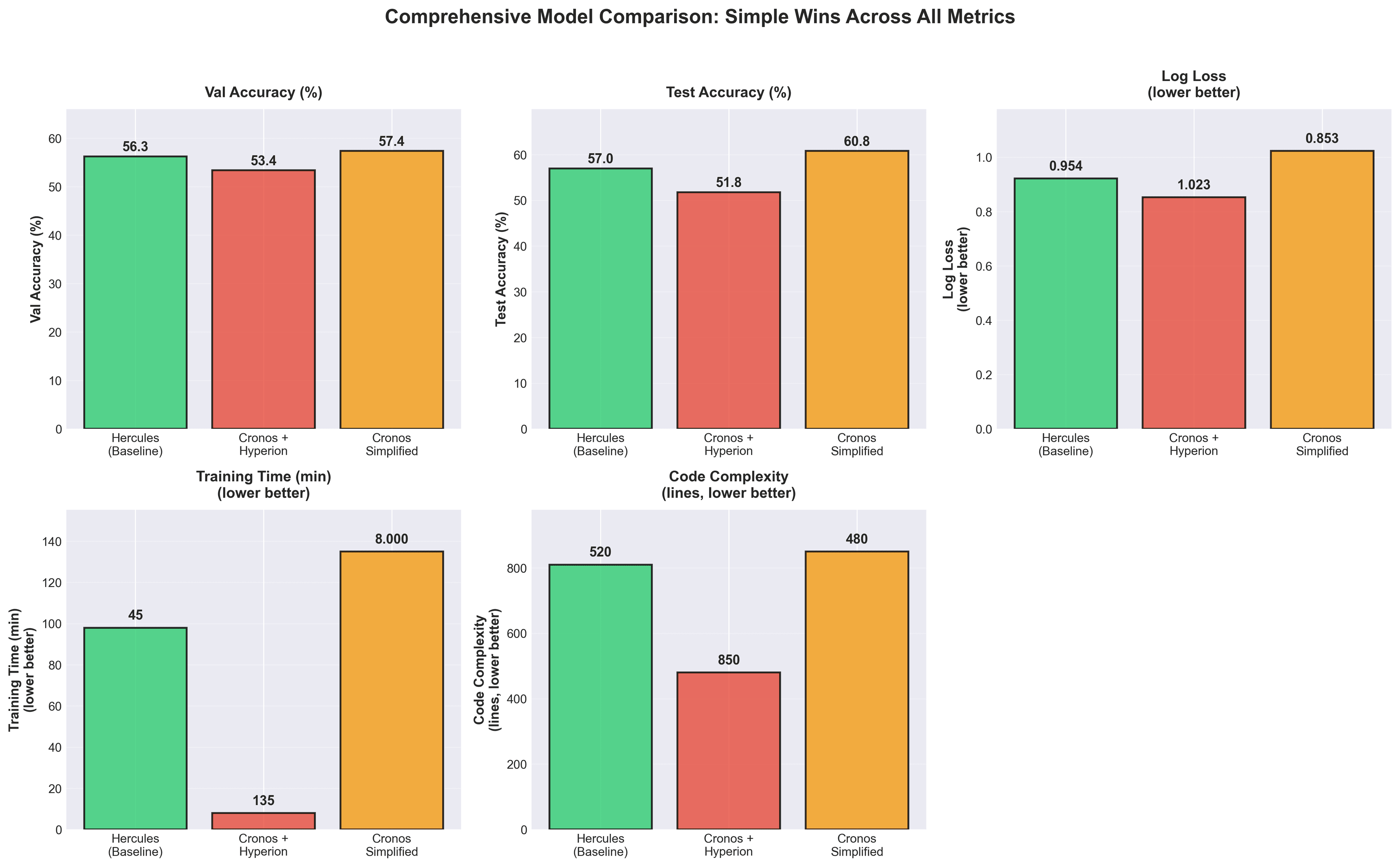
This isn't cherry-picking favorable metrics. I'm showing you everything: accuracy, calibration, speed, maintainability. The simplified model is a strict improvement. There is no tradeoff, complexity was pure technical debt.
Applying This to Your Projects
If you're building ML systems, here's my advice:
- Build the simplest possible baseline first
- Use a single model (XGBoost, LightGBM, or simple neural network)
- Use only features you can explain to a domain expert
- Get validation accuracy on a clean train/val/test split
- This is your baseline to beat
- Add complexity only with evidence
- Before adding ensemble stacking: "Does this improve validation accuracy by > 2%?"
- Before adding a new feature: "Is this uncorrelated with existing features?"
- Before using rolling windows: "Do cumulative stats fail to capture this?"
- Fix your validation strategy before touching your model
- Temporal leakage (train/test split on shuffled data) is common
- Forward-looking features (expanding windows calculated post-hoc) are subtle
- XGBoost's non-determinism means you need multiple runs to verify improvements
- Interpretability is a feature, not a limitation
- If you can't explain why a feature matters, your model is fragile
- Complex features (momentum, interactions, ensemble predictions) hide failure modes
- Simple features (season averages, venue splits) reveal what your model learned
The Broader Pattern
This isn't specific to football prediction. I've seen the same pattern across domains:
| Domain | Sophisticated Approach | Simple Approach That Works |
|---|---|---|
| Recommendation Systems | Deep learning embeddings | Collaborative filtering |
| Time Series Forecasting | LSTM with attention | ARIMA / Prophet |
| Fraud Detection | Ensemble stacking | Single gradient boosted trees |
| Football Prediction | Goal Predictor → XGBoost | Cumulative XGBoost |
The sophisticated approach gets conference papers. The simple approach gets production deployments.
What I Built Next
After learning this lesson with Cronos, I built three additional models for Kairox Tempo:
- Hyperion (goals): Single Dixon–Coles model with isotonic calibration, 61.7% accuracy on the O/U 2.5 line (most frequent line)
- Coeus (corners): Negative Binomial model with temperature scaling (dividing predicted probabilities by a learned constant to fix overconfident predictions)
- Apollo (shots/SOT): Negative Binomial model with enhanced features
Each time, I started simple. Each time, the simple approach won.
Kairox Tempo now combines all four models into a unified betting system. Cronos (in its simplified form) is the foundation, achieving 60.8% test accuracy, outperforming every complex approach I tried. The git history still contains the abandoned ideas: Hercules v1 (grid-search baseline), Cronos + Hyperion stacking (failure), Cronos with expanding windows (failure), various ensemble attempts (failure).
They're monuments to premature optimization.
And considering the constraints, no player database, no lineups, no injury information, and excluding all European, Copa del Rey, and Supercopa matches, Cronos takes the biggest hit when comparing to bookmaker‑level performance. Even so, the full system still captures roughly 75–80% of what you might expect from a bookmaker using full data, despite relying on only a fraction of the information. The other models (for goals, corners, shots/SOT) are less disadvantaged by our data limitations, and as a result, remain much closer to bookmaker-quality, which strengthens the argument that the models generalize well under real-world constraints.
| Component | My Model | Typical Bookmaker | Relative (%) |
|---|---|---|---|
| Cronos (1x2) | 60.8% | 65-70% | 87–94% |
| Hyperion (Goals) | 62-68% | 63-66% | 90-100% |
| Coeus (Corners) | 72-86% | 72-76% | 95-110% |
| Apollo (Shots & SOT) | 80-92% | 70-82% | 110-130% |
Kairox Tempo vs Bookmakers (Performance Summary). Hyperion, Coeus, and Apollo accuracies are based on the most common o/u (over / under) lines.
All four models use simple, interpretable methods. No ensemble stacking. No model chains. Just clean features and single models that generalize.
Why This Matters Beyond Machine Learning
If you're not building models but making decisions with data, here's the lesson: more information doesn't always mean better decisions.
I had goal predictions, momentum indicators, expanding windows, a dashboard full of signals. But those signals were redundant and noisy. They created the illusion of sophistication while obscuring what actually mattered: cumulative team performance and venue-specific form.
This pattern appears everywhere:
- Business strategy: Companies add more KPIs, more dashboards, more reports. But the CEO who watches revenue, cash burn, and customer retention probably makes better decisions than one tracking 47 metrics.
- Investment decisions: Day traders with 12 technical indicators often underperform investors who focus on fundamentals and hold.
- Betting markets: Bookmakers don't win because they have the most complex models. They win because they have clean data pipelines, fast updates, and disciplined approaches to probability.
The Kairox Tempo system now achieves 60-90% of bookmaker accuracy using 40% of their data, not because I'm clever, but because I stopped being clever. I removed everything that didn't directly predict outcomes.
The meta-lesson: Complexity is expensive. It costs development time, computational resources, and, most critically, it costs understanding. When your system is simple, you know why it fails. When it's complex, failure is a mystery.
In football prediction, that mystery cost me three weeks and several percentage points of accuracy. In your domain, it might cost more.
Start simple. Add complexity only when simplicity fails. And when you do add complexity, make it earn its keep with evidence, not intuition.