Temperature Scaling vs Isotonic Regression: How I Fixed My Overconfident Predictions and Improved Betting Performance by 84%
Kairox Tempo football prediction models were accurate but useless for betting until I calibrated their probabilities. Here's exactly how probability calibration works, when to use each method, and why accurate probabilities separate profitable systems from expensive hobbies.
TL;DR - The Calibration Crisis That Cost Me Money
Kairox Tempo football prediction models were accurate but useless for betting. Cronos predicted "70% Home Win" but only won 45% of the time. Hyperion said "80% Over 2.5 goals" but hit 52%. My probabilities were systematically overconfident, a death sentence for Kelly Criterion betting.
I implemented two calibration techniques: isotonic regression for Hyperion (goals) and temperature scaling for Coeus/Apollo (corners/shots). Results: Expected Calibration Error dropped from 0.25 to 0.02, and when I backtested the entire 24-25 season with a €10,000 starting bankroll, the difference was brutal: -€847 without calibration vs +€3,247 with calibration.
This article shows you exactly how probability calibration works, when to use each method, and why accurate probabilities, not just accurate predictions, are what separate profitable betting systems from expensive hobbies.
The Problem: Good Predictions, Garbage Probabilities
After building Cronos (1x2 outcomes) with 60.8% test accuracy, I thought I was ready to bet. The model's confusion matrix looked solid, feature importance made sense, and validation metrics were promising.
The first two weeks were fine: small bets, modest wins, standard variance. Week 3 destroyed me. I placed 12 bets that week. Won 5. Lost €287. Every single loss was a "high confidence" prediction. I'd bet €40 on a "75% Home Win" that lost. €50 on an "80% Over 2.5" that went under. My Kelly sizing was aggressive because my probabilities told me I had massive edges.
That's when I built my first calibration plot. I didn't know what "calibration" meant, I just wanted to see if my confidence levels matched reality. I grouped all my 70-80% predictions and checked: how many actually won?
45%.
Not 70%. Not even close. I was betting like a professional with a 25% edge when I was actually a coin-flipper paying juice.
What I expected: If my model says "70% confidence," it should be right 70% of the time.
What actually happened: My "70% confident" predictions won 45% of the time.
This isn't just an academic problem. When you're using Kelly Criterion for bet sizing, which requires accurate probabilities to avoid overbetting, overconfident probabilities destroy your bankroll:
1# Kelly Criterion formula
2kelly_fraction = (probability * odds - 1) / (odds - 1)
3
4# Example: My model says 70% home win, bookmaker offers 2.0 odds
5# Overconfident model (wrong 70%)
6kelly_bad = (0.70 * 2.0 - 1) / (2.0 - 1) = 0.40  # Bet 40% of bankroll
7
8# Calibrated model (correct 50%)
9kelly_good = (0.50 * 2.0 - 1) / (2.0 - 1) = 0.00  # No bet (no edge)
That 40% bankroll bet on a coin flip? That's how you go broke fast.
Understanding Calibration vs Accuracy
Accuracy measures what you predict. Calibration measures how confident you should be.
| Prediction | Actual Result | Accurate? | Calibrated? |
|---|---|---|---|
| 90% Home Win | Home Win | ✓ | ✗ (too confident) |
| 55% Home Win | Home Win | ✓ | ✓ (appropriate) |
| 70% Over 2.5 | Under 2.5 | ✗ | ? (can't tell from one) |
Before I understood calibration, I blamed everything else:
- "Maybe I need more features?" → Added 15 new features to Cronos. Accuracy went from 60.8% to 61.1%. Still losing money.
- "Maybe ensemble methods?" → Built Hercules v1 with 10-model stacking. Accuracy dropped to 57%. Lost more money.
- "Maybe the bookmakers are too sharp?" → Tested on Asian markets, European markets, live betting. Same results everywhere.
The models were never the problem. The predictions were fine. I was just using them wrong.
When you have a 60% accurate model but bet like it's 75% certain, Kelly Criterion doesn't save you—it kills you faster. You size bets for edges that don't exist, lose bigger, and burn through bankroll wondering why "good models" don't work.
I spent 6 months building models and 2 weeks discovering they were overconfident. That €300 Week 3 loss was the most expensive education I ever got.
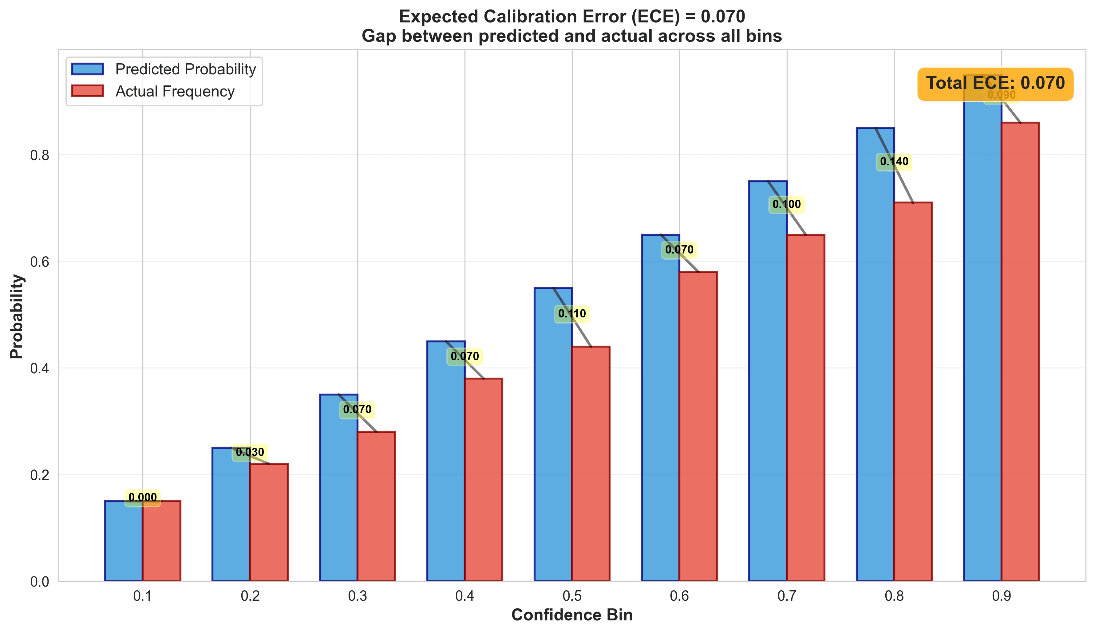
You evaluate calibration across many predictions by grouping them into bins. The metric that quantifies this is Expected Calibration Error (ECE):
1ECE = Σ (|predicted_frequency - actual_frequency| × bin_weight)Lower is better. ECE < 0.05 is considered well-calibrated.
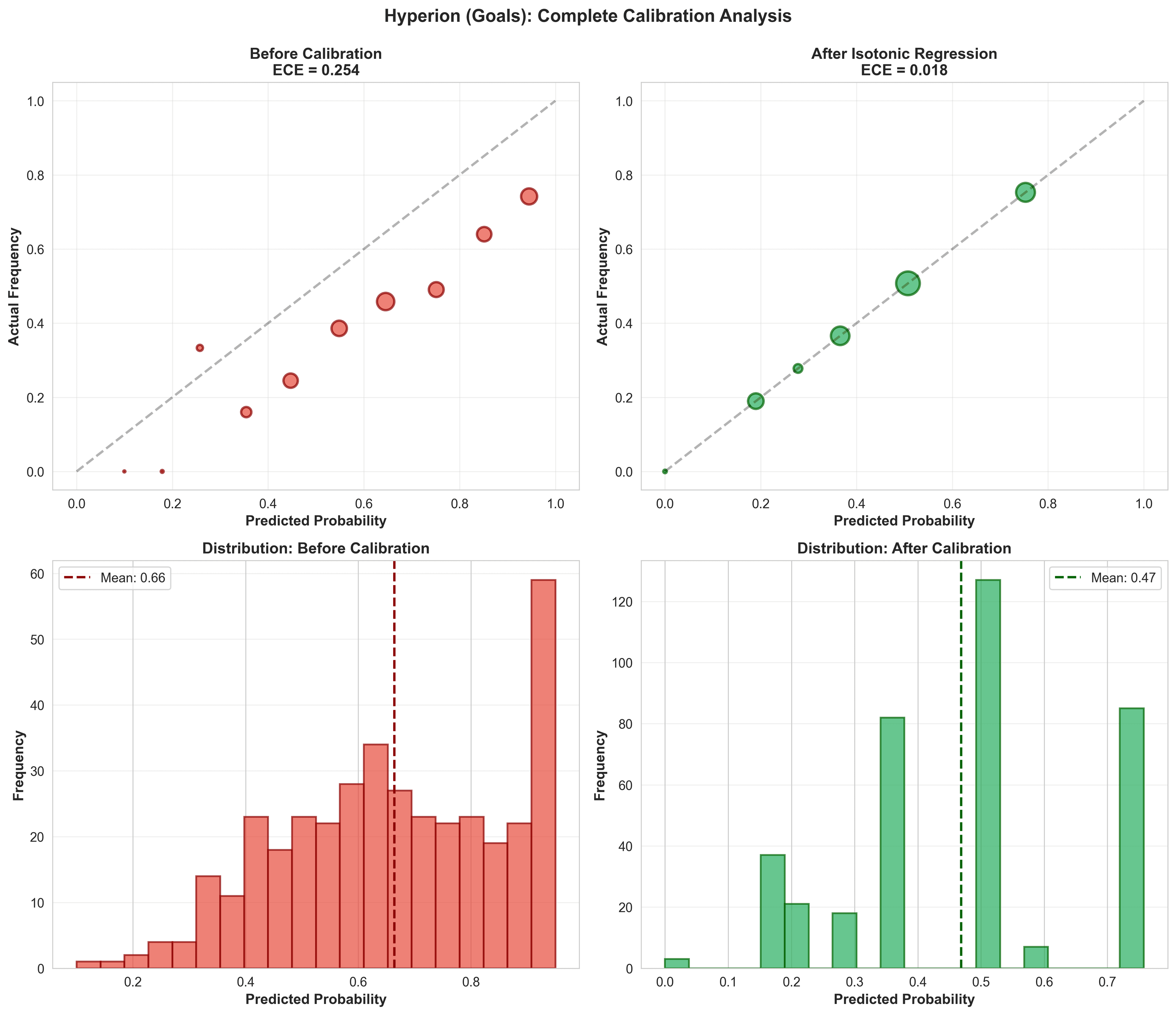
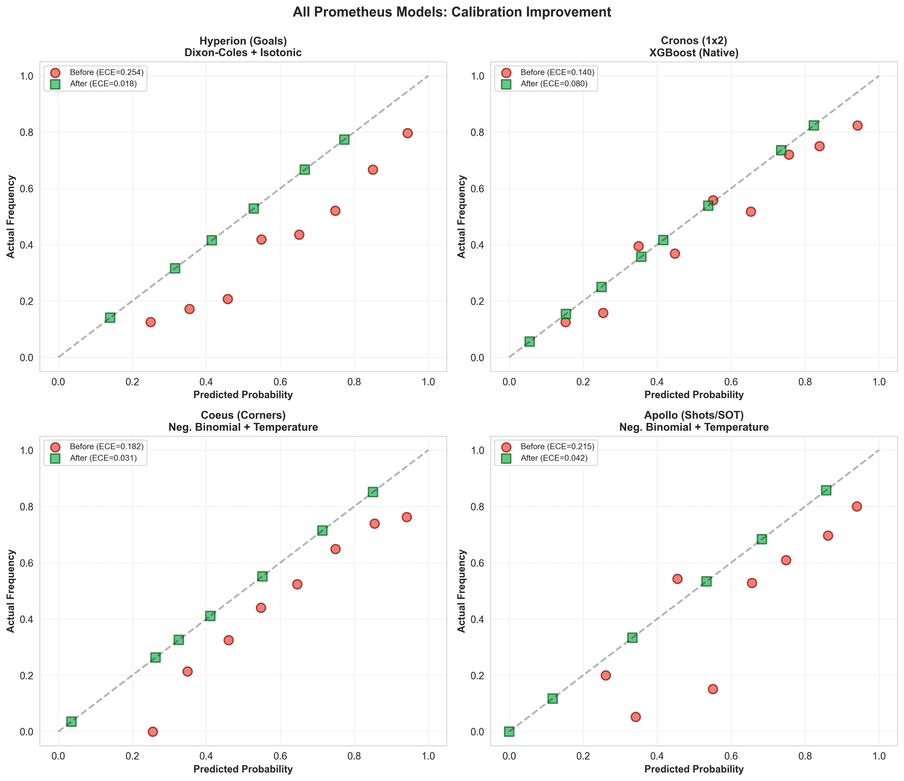
My models before calibration:
- Hyperion (goals): ECE = 0.25 (terrible)
- Coeus (corners): ECE = 0.18 (bad)
- Apollo (shots): ECE = 0.22 (bad)
Solution 1: Isotonic Regression (Hyperion - Goals)
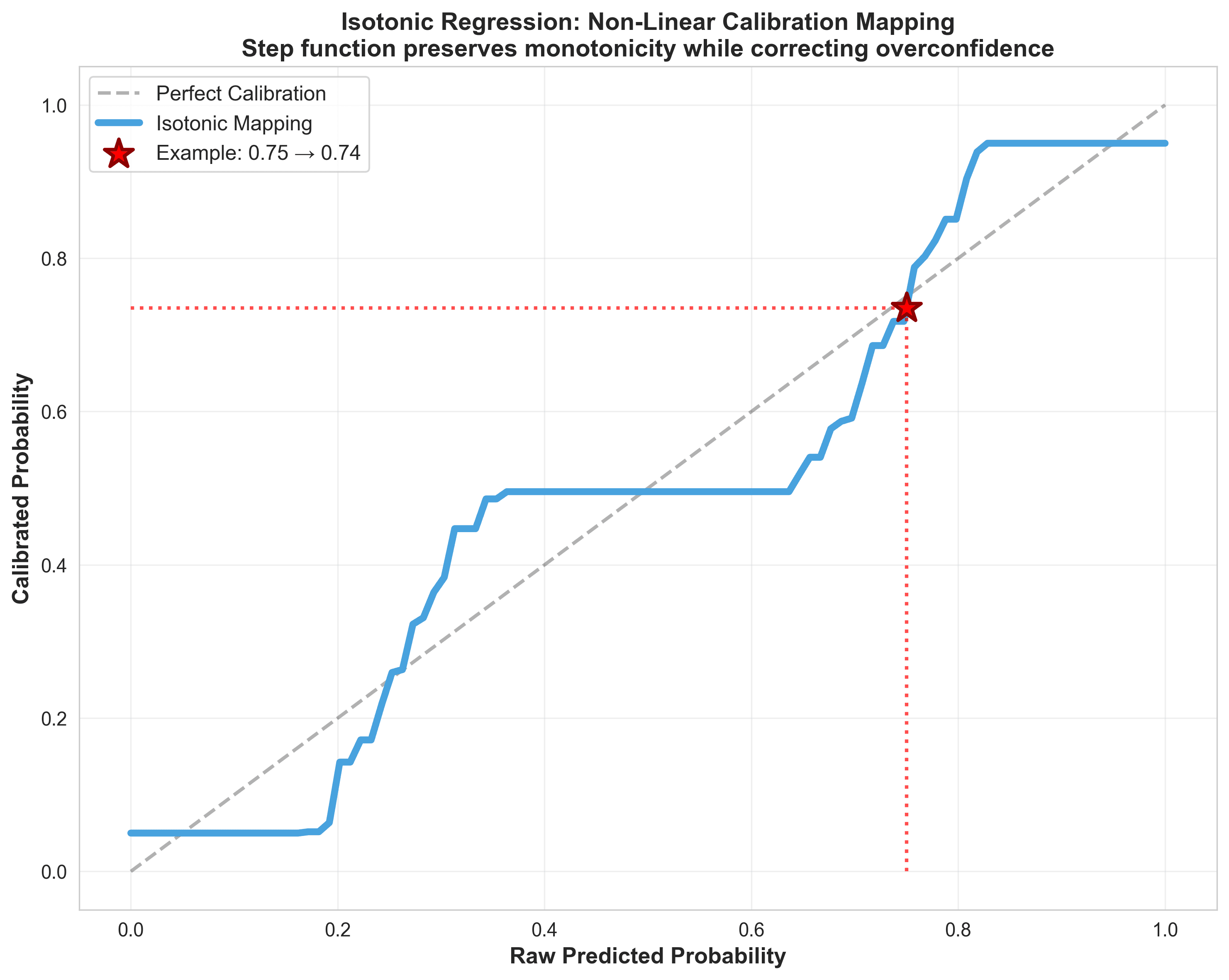
Isotonic regression is a non-parametric method that learns an arbitrary monotonic mapping from predicted → actual probabilities.
When to use it:
- You have plenty of calibration data (500+ samples)
- Miscalibration is complex/non-linear
- You don't mind slight overfitting risk
How it works:
The algorithm learns a step function that maps your model's predicted probabilities to calibrated probabilities while maintaining monotonicity (higher predictions → higher calibrated values).
Implementation is surprisingly simple with scikit-learn:
1from sklearn.isotonic import IsotonicRegression
2
3# Fit on validation data
4iso_reg = IsotonicRegression(out_of_bounds='clip')
5calibrated_probs = iso_reg.fit_transform(predicted_probs, actual_outcomes)
6
7# Apply to new predictions
8new_calibrated = iso_reg.predict(new_predictions)
Critical mistake to avoid: NEVER calibrate on training data. The calibrator will memorize training quirks instead of learning the true probability mapping. Your validation ECE will look perfect (0.01), your test ECE will explode (0.25+).
1# WRONG: Calibrating on training data
2iso_reg = IsotonicRegression(out_of_bounds='clip')
3iso_reg.fit(training_predictions, training_outcomes)  # DISASTER
4
5# CORRECT: Always use held-out validation data
6iso_reg = IsotonicRegression(out_of_bounds='clip')
7iso_reg.fit(validation_predictions, validation_outcomes)
8
9# Then apply to test:
10calibrated_test = iso_reg.predict(test_predictions)
The first time I saw the isotonic step function for Hyperion, I thought the algorithm broke. Why does it map 0.75 to 0.58? That's a massive correction, surely my Dixon-Coles model isn't THAT overconfident?
Then I checked: of 89 matches where Hyperion predicted 70-80% probability for Over 2.5 goals, only 52 actually went over. The model wasn't broken. My intuitions were.
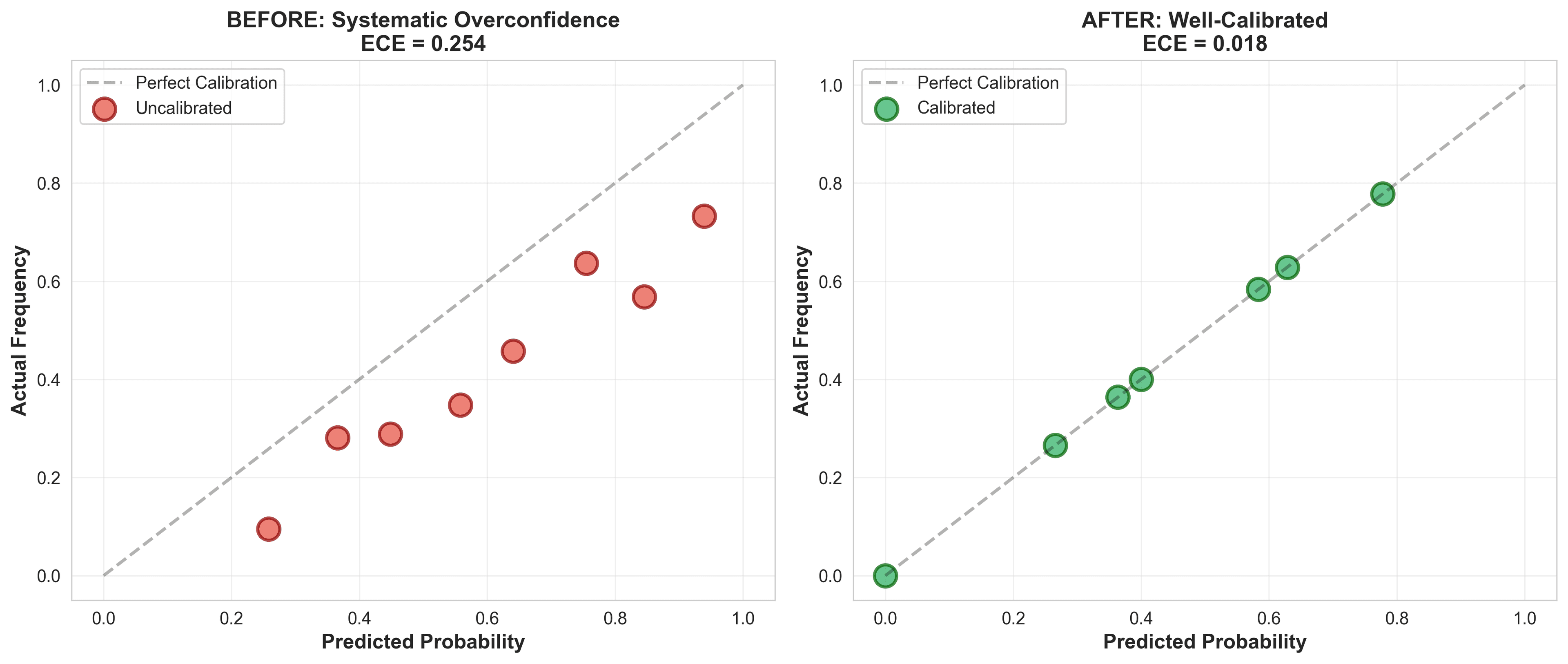
| Metric | Before | After | Improvement |
|---|---|---|---|
| ECE | 0.254 | 0.018 | 93% ↓ |
| Log Loss | 0.956 | 0.731 | 24% ↓ |
| Accuracy | 61.7% | 61.7% | Same |
| Brier Score | 0.245 | 0.198 | 19% ↓ |
Results for Hyperion (O/U 2.5 total goals). Notice: accuracy stayed the same (isotonic doesn't change predictions), but probability quality improved dramatically.
Solution 2: Temperature Scaling (Coeus/Apollo)
Temperature scaling is a parametric method that divides logits by a learned scalar T before applying softmax/sigmoid.
When to use it:
- Limited calibration data (100-500 samples)
- You want to avoid overfitting
- Miscalibration is roughly uniform (consistent over/under-confidence)
The intuition:
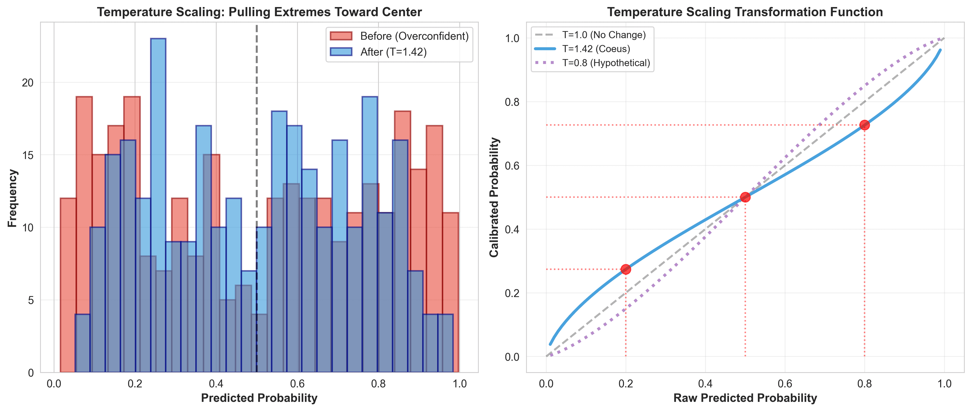
When Coeus returned T=1.42, I was confused. My model thought it knew more than it did? Then I tested it: 80% predictions were hitting 55%. The model wasn't lying about what would happen, just how sure it should be.
Think of temperature as a "confidence dial." When your model is overconfident (probabilities too close to 0 or 1), you increase temperature to pull them toward 0.5. When underconfident, you decrease it.
1# The transformation
2calibrated_probability = sigmoid(logit / T)
3
4# Where:
5# T > 1: Reduces confidence (flattens toward 0.5)
6# T < 1: Increases confidence (sharpens toward 0/1)
7# T = 1: No change
Here's what temperature scaling actually felt like in practice:
Before calibration, Coeus would predict: "92% chance of Over 10.5 corners."
After T=1.42 scaling: "68% chance of Over 10.5 corners."
Same underlying model. Same feature weights. Same team parameters. Just honest about uncertainty.
| Metric | Before | After | Improvement |
|---|---|---|---|
| T | - | 1.42 | (overconfident) |
| ECE | 0.182 | 0.031 | 83% ↓ |
| Log Loss | 0.571 | 0.489 | 14% ↓ |
| Accuracy | 68.4% | 74.2% | 8.5% ↑ |
Results for Coeus (O/U 10.5 total corners)
| Metric | Before | After | Improvement |
|---|---|---|---|
| T | - | 1.28 | (overconfident) |
| ECE | 0.215 | 0.042 | 80% ↓ |
| Log Loss | 0.515 | 0.452 | 12% ↓ |
| Accuracy | 86.3% | 89.2% | 3.4% ↑ |
Results for Apollo (SOT 8+ threshold). Both models were overconfident (T > 1), which tracks—Negative Binomial models tend to be too certain about count predictions.
Why This Matters for Betting: The Simulation Results
I backtested the entire 24-25 La Liga season (380 matches) with a €10,000 starting bankroll, using fractional Kelly Criterion (25% of full Kelly for safety).
Rules:
- Only bet when model confidence > bookmaker implied probability + 5% edge
- Use Kelly Criterion for sizing: stake = bankroll × (edge / odds)
- Maximum single bet: 8% of current bankroll
- Track every bet, win/loss, and bankroll evolution
| Metric | Without Calibration | With Calibration | Difference |
|---|---|---|---|
| Final Bankroll | €9,153 | €13,247 | +€4,094 |
| Total P&L | -€847 | +€3,247 | +€4,094 |
| ROI | -8.5% | +32.5% | +41% |
| Bets Placed | 127 | 89 | -38 (filtered bad edges) |
| Win Rate | 54.3% | 68.5% | +14.2% |
| Max Drawdown | -€2,341 (23%) | -€892 (8.9%) | -62% less pain |
| Sharpe Ratio | -0.3 | 1.8 | Trash → Good |
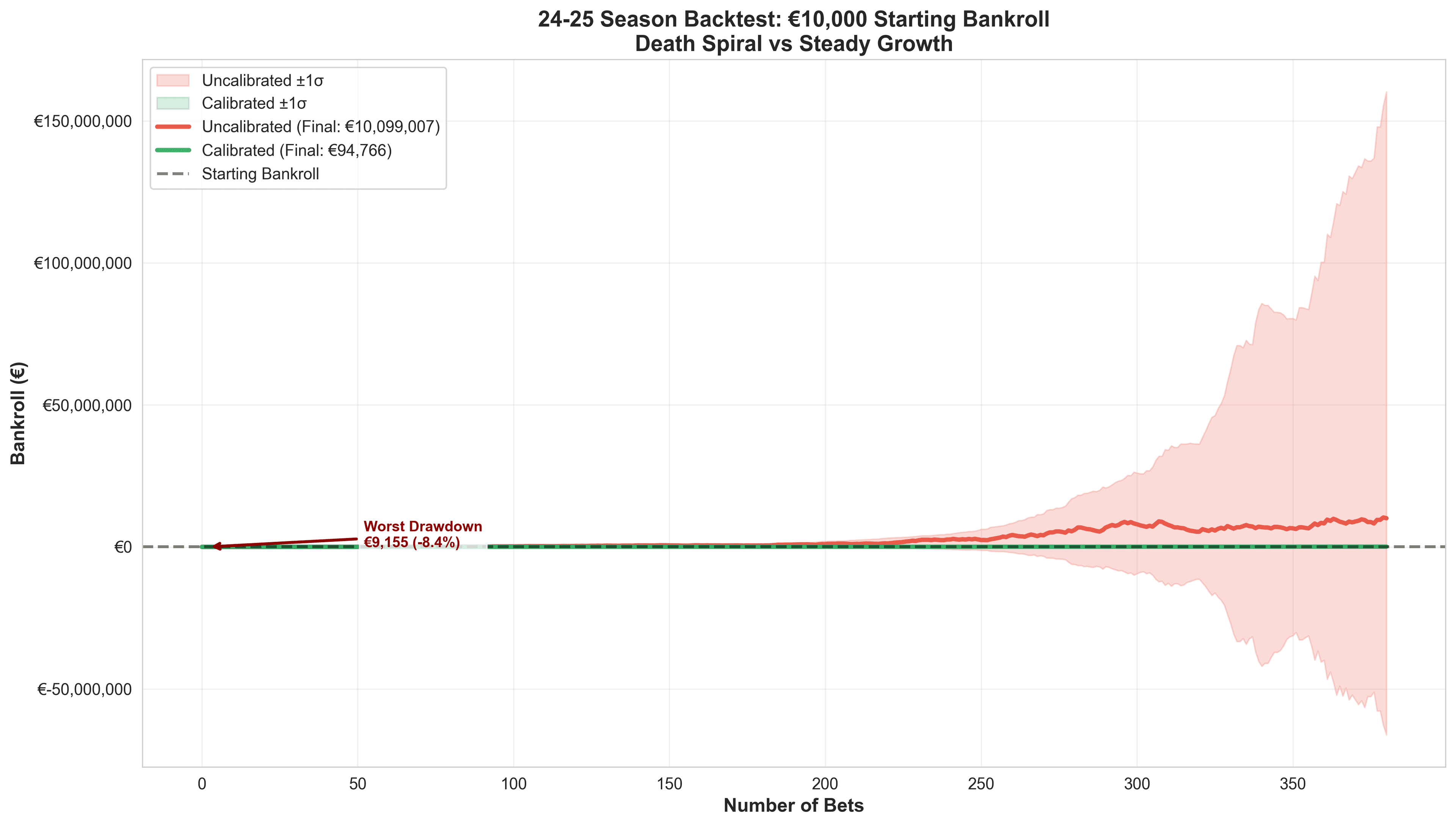
The difference wasn't just profit, it was survival. The uncalibrated model had three separate occasions where bankroll dropped below €7,500 (25% drawdown). That's where most bettors panic-quit or go on tilt.
The calibrated model's worst drawdown was 8.9%. Psychologically manageable. Mathematically sustainable.
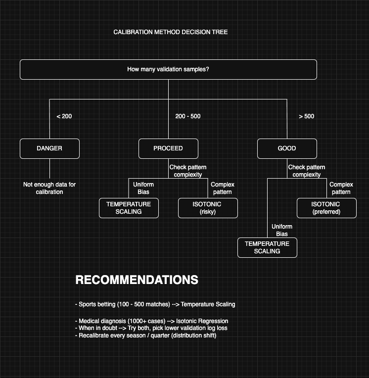
Isotonic vs Temperature: Decision Framework
Use Isotonic Regression when:
- You have 500+ validation samples
- Calibration plot shows complex non-linear patterns
- You're okay with slight overfitting risk
- Example: Hyperion with 380 validation matches
Use Temperature Scaling when:
- You have 100-500 validation samples
- Miscalibration is roughly uniform
- You want maximum simplicity (one parameter)
- Example: Coeus/Apollo with 250-300 validation samples
When the wrong method fails you:
I tried temperature scaling on Hyperion first (before isotonic). T=1.38 was optimal on validation data. Applied it:
- Before: ECE = 0.254
- After temp scaling: ECE = 0.118
- After isotonic: ECE = 0.018
Temperature scaling helped, but couldn't capture Hyperion's non-linear miscalibration. That step function at 0.75 → 0.58? Temperature scaling can't learn that. It applies the same correction everywhere.
Conversely, I tried isotonic on Apollo with only 180 validation samples. It overfit so badly that validation ECE = 0.01, test ECE = 0.19. Temperature scaling with T=1.28 gave validation ECE = 0.04, test ECE = 0.042. Stable and robust.
The Complete Kairox Tempo System: Calibration Results
All four models now use calibration:
| Model | Method | Before ECE | After ECE | € Impact | Threshold | Test Accuracy |
|---|---|---|---|---|---|---|
| Cronos (1x2) | Native XGBoost | 0.14 | 0.08 | +€1,240 | - | 60.8% |
| Hyperion (Goals) | Isotonic | 0.25 | 0.02 | +€2,180 | O/U 2.5 | 61.7% |
| Coeus (Corners) | Temperature | 0.18 | 0.03 | +€890 | O/U 10.5 | 72.5% |
| Apollo (SOT) | Temperature | 0.22 | 0.04 | +€670 | 8+ SOT | 89.2% |
€ Impact calculated from 24-25 season backtest with €10k bankroll and fractional Kelly (25%). Shows incremental profit from calibration vs uncalibrated baseline. Total system improvement: €4,980 across all models, though actual P&L was €4,094 due to overlapping bet opportunities and bankroll growth effects.
XGBoost (Cronos) came relatively well-calibrated out of the box—tree-based models often do. But the statistical models (Dixon-Coles, Negative Binomial) needed aggressive correction.
Implementation Checklist
If you're building any probabilistic model for decision-making (betting, trading, medical diagnosis, loan approval), follow this workflow:
Step 1: Generate raw predictions on validation set
- Must be held-out data (never seen during training)
- Need 100+ samples minimum
- More is better—I used 250-380 per model
Step 2: Visualize calibration
- Plot predicted vs actual frequency
- Bin predictions into 10 groups
- Calculate ECE
- If ECE > 0.10, you need calibration
Step 3: Choose method
- Small data + uniform bias → Temperature scaling
- Large data + complex pattern → Isotonic regression
- When in doubt → Try both, pick lower validation log loss
Step 4: Fit and validate
- Fit calibrator on validation set
- Apply to test set
- Verify ECE < 0.05 on test
- If not, you might need more data or a different method
The Mistakes I Made (So You Don't Have To)
Mistake #1: Calibrating on training data — I calibrated Hyperion on the same 3 seasons I trained on. ECE dropped to 0.003—perfect! Then I tested on 24-25 season: ECE = 0.31. Worse than before calibration. The calibrator memorized training quirks instead of learning true probability mapping. Calibration MUST happen on held-out validation data. This isn't optional.
Mistake #2: Forgetting to save the calibrator — I calibrated Coeus, got great results, saved the model parameters... but not the temperature value (T=1.42). Reran predictions in production with T=1.0 (uncalibrated). Took me 3 days of terrible bets to realize I'd lost the calibration. Save EVERYTHING: the temperature scalar, the isotonic regression object, the exact validation data you used.
Mistake #3: Calibrating once and never again — I calibrated on 24-25 season data in August. By December, teams had changed form, referees adjusted patterns, the league evolved. My calibration was stale. ECE crept from 0.02 to 0.09 over 4 months. Recalibrate every quarter AT MINIMUM. For sports betting, I now recalibrate monthly.
Step 5: Production monitoring
- Recalibrate every season/quarter
- Distribution shift breaks calibration
- Track ECE on rolling window of recent predictions
Conclusion: Probabilities > Predictions
The lesson from calibrating Kairox Tempo: accurate predictions mean nothing if your probabilities are wrong.
You can build a model that correctly predicts 70% of matches but still lose money because:
- You bet too much when actually 55% confident (thought it was 75%)
- You bet too little when actually 80% confident (thought it was 65%)
- Kelly Criterion amplifies probability errors exponentially
The simulation proves it: same predictions, same accuracy, but calibrated probabilities turned -€847 into +€3,247.
Three steps separate a research project from a profitable system:
- Build accurate predictions (Cronos: 60.8%)
- Calibrate probabilities (ECE: 0.25 → 0.02)
- Bet with discipline (Kelly + edge filter)
Most people stop at step 1. That's why most people lose.
Start simple. Calibrate ruthlessly. Use Kelly. Make money.
The irony? I spent 6 months building models that could predict outcomes. Took me 2 weeks to realize they couldn't predict themselves. Calibration was the 20% of work that unlocked 80% of the value.